Mitchell Tutorial: Gradient Boosted Decision Trees

This tutorial will walk you through the process of implementing an algorithm for gradient boosted decision trees in Mitchell. This implementation will make use of the Mitchell Classification and Regression Trees (CART) and Decision Tree libraries, as well as the LibSVM-compatible file reader from the Mitchell IO libraries.

Background
Building a Gradient Boosting Implementation
1. Parsing
2. Implementing the Algorithm
The Complete Program

Background

What are Decision Trees?

A decision tree is a tool for classifying something based on a finite set of features. We will be working with decision trees that map features to real values.

For example, the following decision tree can be used to determine the probability that someone has the flu:

Decision Tree Example

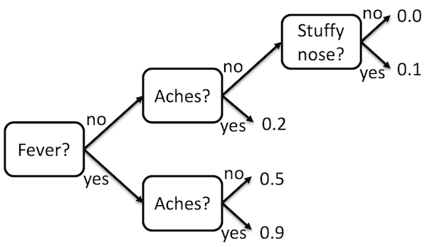
The tree is read from left to right. At each point in the tree a feature is examined to determine which way to go. The results are stored at the leaves.

The Mitchell Decision Tree Libraries

Mitchell includes two libraries for the representation decision tree libraries: one for real-valued features and labels and one for integer-valued features and labels. We will be using the tree for real-valued features and labels.

To use values, functions, and types from the decision tree library, you have three choices. You can prefix the values, functions, and types with the module name, like DecisionTreeReal.forward. If the name is too long, you can give it a shorter name by writing

structure D = DecisionTreeReal;

Then you will be able to write D.forward. Or, if you don’t want to prefix the names at all, you can write

open DecisionTreeReal;

We recommend using one of the first two options, because names in different modules can clash otherwise.

The decision tree itself is represented using the following datatype:

datatype dt = Lf of label | Nd of dt * feature * dt;

dt is the type for decision trees. A value of type dt can be one of two things: a leaf of the tree or an internal node of the tree. Lf and Nd are constructors used to create leaves and internal nodes, respectively.

A leaf node contains the label that the decision tree decides belongs to the object. The internal node contains the feature value. If the feature value is greater than the feature of the object, the left branch is taken. If the feature value is less than the feature of the object, the right branch is taken.

The label type is declared just before dt in the library as a synonym for a real number. Similarly, the feature type is declared as a synonym for a pair of an integer (the feature identifier) and a real number (the feature value).

type label = real;
type feature = int * real;

To create a decision tree by hand, you would write

val myleaf1 = Lf 0.7;
val myleaf2 = Lf 0.0;
val mynode = Nd (myleaf1, (2, 1.0), myleaf2);

or on one line

val mynode = Nd ((Lf 0.7), (2, 1.0), (Lf 0.0));

Then mynode is the decision tree that you have defined. In order to look inside of mynode, you use a case expression (which is different from a case statement in language like C and Java):

(* This is Mitchell comment syntax. *)
val result =
  case mynode of
      Lf lab => ("A leaf label", lab) (* This is a pair of a string and a real. *)
    | Nd lhs (featureId, featureVal) rhs => ("A feature value", featureVal)

The result value will be ("A feature value", 1.0). We will see how to look all of the way down a tree (rather than just at one node) a little bit later in this tutorial.

The decision tree library also includes several functions for using decision trees. We will explain those as we use them. You can also read about them in the documentation.

The Mitchell CART Libraries

Mitchell has a library for creating decision trees from data using CART.

There are two CART implementations, one for working with integer-labeled decision trees and one for working with real-labeled decision trees. We will be using CartReal, which works with real-labeled decision trees. CartReal can work with any real-labeled, real-featured decision tree implementation, so we have to pick which one we will use before we can use CartReal. Modules that can work with multiple implementations of other data structures like this are called functors.

To specify that we want to use CartReal with DecisionTreeReal, we do something similar to how we defined a shorter name for DecisionTreeReal.

structure C = CartReal(structure D = DecisionTreeReal);

If you don’t want to prefix things with C., you can write

structure C = CartReal(structure D = DecisionTreeReal);
open C;

to import everything.

Of particular interest in CartReal is the function train, which has type (D.features * D.label) list -> D.t. Here D is short for the kind of decision tree we told CartReal to use.

To the left of the arrow are the types of the inputs to the function, in the form of a pair. A pair type is also known as a “product type”, hence the use of the infix * to form the type of a pair with D.features on the left and D.label on the right. To the right of the arrow is type of the output.

In Mitchell some types, like list, work with other types. For example, a list of integers would have type int list. In this case, the input to train is a list of pairs, where the left-hand-side of the pair has feature information, and the right-hand-size has labels.

Earlier we said the definitions for the D.feature and D.label types:

type label = real;
type feature = int * real;

This function uses the D.features (not the same as D.feature, note the “s”!) type, which is defined as an array of integers (array is like list, in that it works with other types):

type features = int array;

The CART library requires that all of the training data use arrays of the same size. That is, every feature array must have the same value for Array.length. The length of an array is specified by the first argument to Array.array when creating an array containing all the same value, by the first argument to Array.tabluate when defining array using the value of a function applied to each of its indices, or by the length of the list to be converted to an array using Array.fromList.

What is Gradient Boosting Decision Trees?

Gradient boosting is a way of combining lots of weak classifiers (such as decision trees) to make a strong classifier. See here for a a general description of gradient boosting.

For decision trees, first, we train a decision tree on some data, and scale the predictions of the decision tree by a parameter called the learning rate. That decision tree will have a large amount of error. We compute the difference between the predictions of the decision tree on the data and the actual labels on the data. These differences are called the residuals.

To account for the error of the first decision tree, we train a new decision tree on the residuals, and again scale by the learning rate. To compute the predictions of the collection (or ensemble) of decision trees, we take the sum of the predicted values. We repeat this process for some number of decision trees.

This process continues until we meet some stopping criteria, such as the number of decision trees we want in our ensemble.

The Mitchell Gradient Boosted Decision Trees Library

Mitchell has a library for Gradient Boosted Decision Trees, as well as a library for reading input to train and test the ensembles of decision trees. To use the library, first import the modules:

structure C = CartReal(structure D = DecisionTreeReal);
structure Gbdt = Gbdt(structure CART = C);
structure G_IO = LibSVMReader;

To read input in the format

2:1 5:1 6:1
2:1 6:1 12:1
3:1 5:1 12:1 13:1

where the first number is the label for an object, and the rest of the entries are the feature number and value separated by a colon, use

val trainingData = G_IO.fromFile "/data/workload33-gbdt/agaricus.txt.train";
val testData = G_IO.fromFile "/data/workload33-gbdt/agaricus.txt.test";

To train the ensemble of trees and print the ensemble

val gbdt = Gbdt.train (trainingData, 0.8, 2);
val _ = print (Gbdt.toString gbdt);

If you use the input format example above as the training data, you will get the rather uninteresting result of an ensemble of three single-node trees. Single node trees just predict a single number, without looking at the features. They arise in this case because of the limited amount of data used to train the decision trees.

You can find more interesting data in /data/workload33-gbdt/ or you can find datasets online, such as here.

To test the ensemble of trees and print the error

val error = Gbdt.error (gbdt, testData);
val _ = print ("error = " ^ (Real.toString error) ^ "\n");

Building a Gradient Boosting Implementation

We will now walk through using the CartReal and DecisionTreeReal libraries to build the GBDT algorithm from scratch.

You can find training data to use for this tutorial workload here. This tutorial will assume you have downloaded the training data into the directory /data/workload33-gbdt/.

Parsing

We are in the process of developing Mitchell libraries for ingesting data in many common formats. As shown above, the input format used for gradient boosting decision trees is one of the formats for which we have library support.

Note that you will not have to implement any parsing code for your assigned workload. The data preparation and parsing has been done for you as part of the scaffolding for the assigned workload. However, you may find it useful practice with the language to implement your own parser in Mitchell before beginning working on the assigned workload.

If you are going to implement your own parser, we recommend using a language other than Mitchell for preparing the data for use by Mitchell, and then implementing a simple data ingesting function using the TextIO and TextIO.StreamingIO modules to read the data into a string, and then parsing it with the functions from Substring module, such as Substring.tokens.

See the tuorial on IO and parsing in Mitchell for more information.

Implementing the Algorithm

First, import the libraries that we will be using

structure C = CartReal(structure DT = DecisionTreeReal);
structure D = C.DT;

Gradient-boosting produces an ensemble of decision trees. We are going to represent the ensemble as a list D.t list. D.t is the type of a single decision tree.

Forward

First we will implement the forward-mode, prediction function for the ensemble of decision trees. This involves applying the D.forward function to each decision tree in the ensemble, and then summing the results. Mitchell includes some helper functions and other features to make it easier for us to implement this. Our forward function will have the type

(D.t list * D.features) -> real

That is, forward takes the ensemble and the features of the object to predict, and produces a real number prediction.

To define forward we will use a let construct, which lets us define local variables and helper functions that use the arguments to forward. The value of the expression between in and end is the result of the whole let expression.

fun forward (ensemble, features) =
    let
      fun forwardTree tree = D.forward (tree, features);
      val predictions = List.map forwardTree ensemble;
    in
      MathReal.sum predictions
    end;

First, we define forwardTree, which is a function that takes a tree and applies D.forward to it and the features. Then we use the library function List.map to apply the forwardTree function to each of the trees in the ensemble. The result of this is a list of predictions (predictions: real list, read the colon : as “has type”). then we produce the final result by summing the predictions.

List.map is a little different from other functions we have seen: rather than taking its arguments in a tuple (like a pair), it takes its arguments separately. Many of the functions from the subset of the Standard ML Basis Library that is available in Mitchel will take arguments in this way. The difference is mostly for convenience (taking the argument separately allows one to partially apply the function), but we will not use any of those conveniences in this tutorial and you do not need to use them in your code.

Loss Function

Next, we will implement the loss function. This takes an ensemble, features, and the true label, and determines how far off the prediction is.

fun lossR (ensemble, features, actualLabel) =
    let
      val predictedLabel = forward (ensemble, features);
    in
      actualLabel / (1.0 + Math.exp(actualLabel * predictedLabel))
    end;

Scaling

One of the operations we have to perform on the decision trees is to scale the predictions by a learning rate. This function will crawl the tree to find the leaves, and then build the tree back up with scaled predictions at the leaves.

There are two interesting things about how we implement this function. First, we implement the recursively, that is, in terms of itself. This works because each internal node (D.Nd) has two smaller trees inside of it (lhs and rhs). We can keep calling scale until we hit the smallest tree, a leaf (D.Lf, which has no sub-trees), and everything bubbles back up.

The second interesting thing we do is use a helper function to implement scaleLeaves. The helper function allows us to focus on the parts of the program that change on each call (which sub-tree scale is being called on), rather than on the parts that stay the same (the learning rate).

The scaling itself happens at the leaves, producing a new leaf with the predicted label multiplied by the learning rate.

fun scaleLeaves (tree, learningRate) =
  let
    fun scale tree =
      case tree of
          D.Lf label => D.Lf (label * learningRate)
        | D.Nd (lhs, feature, rhs) => D.Nd ((scale lhs), feature, (scale rhs));
  in
    scale tree
  end;

Training the Next Tree

When training a tree, one of the things we want to do to prevent over-fitting is to prune the tree, and then select the tree that has the most leaves, but no more leaves than the average number of nodes in all of the trees so far. To select the best tree, we write a function that compares two trees based on the number of leaves.

fun compareLeaves (avg, left, right) =
    if (D.leafNum left < avg) andalso (D.leafNum left > D.leafNum right)
    then GREATER
    else LESS;

The return type order can be one of GREATER, LESS, or EQUAL, which stand for “greater than”, “less than”, and “equal to”, respectively. Here we return GREATER for the tree that we prefer.

We then use the comparison function to define a function that gets the “best” tree from a list of trees.

fun findBest trees =
    let
      val avg = MathInt.average (List.map D.leafNum trees);
      fun comp (left, right) = compareLeaves (avg, left, right);
    in
      Ord.argmax comp trees
    end;

Like in earlier code snippets, we define a helper function that uses a value that we computed.

The findBest function uses the Ord.argmax function to pick the best item from the list, according to the comparison function that has been defined using the average number of leaves in the trees. Ord.argmax returns a value of type D.t option, which can be one of two things. If the list given to Ord.argmax is empty, then the result is NONE. Otherwise the list will be SOME t, where t is the chosen tree.

Now we can define the function for computing the next tree to add to the ensemble. This function builds on all of the techniques we’ve talked about so far to train a new tree according to the algorithm.

fun calculateNextTree (ensemble, data, learningRate) =
    let
      fun lossForEnsemble (features, label) = lossR (ensemble, features, label);
      fun lossWithFeatures (features, label) = (features, lossForEnsemble (features, label))
      val residuals = List.map lossWithFeatures data;
      val trainedTree = C.train residuals;
      val prunedTreesWithEvaluationValue = C.prune (trainedTree, data);
      val prunedTrees = map #2 prunedTreesWithEvaluationValue
      val best = findBest prunedTrees;
      val bestTree = case best of NONE => trainedTree | SOME t => t;
    in
      scaleLeaves (bestTree, learningRate)
    end;

Finally, to train the whole ensemble, we need to take the number of trees we want the ensemble to have and the learning rate that we will scale each tree by. To implement this we use recursion again, but this time instead of calling the function on a smaller tree each time, we will call it with a smaller depth each time, until the depth hits zero.

To do this, we check the if the depth is zero. If it is (the then case), we return a simple decision tree that just predicts the average label for everything. If it is not zero (the else case), we ask for the ensemble trained to a depth of one less than the current depth, and then train the tree for the current depth on the residual for the ensemble.

This code snippet also shows how arbitrary expressions can go in the conditional or branches of an if expression. let ... in ... end is an expression like any other (whose value happens to be the value of the expression between in and end), and so can be used as a branch of the if expression. We have to nest the call to train within a branch of the if expression because otherwise we’d have an infinite recursive call (i.e., an infinite loop).

fun train (data, learningRate, depth) =
    if depth = 0
    then [D.Lf (MathReal.average (List.map #2 data))]
    else
      let
        val ensemble = train (data, learningRate, depth - 1);
        val nextTree = calculateNextTree (ensemble, data, learningRate);
      in
        nextTree::ensemble
      end;

Here, the square brackets are how you write a list in Mitchell. The list in the program contains a single element, which is a leaf node that returns the average of the labels on the data.

The #2 is the function that gets the second element of a tuple (e.g., the right-hand side of a pair). Even though #2 starts with a symbol, it is a normal function. If you want to pass an operator (like +) as an argument, you need to prefix it with op, as in op+.

The :: at the end makes a new list out of the existing ensemble (which is represented as a list) and the next tree to add to it. Since the ensemble is used by summing the results of applying the individual trees, it doesn’t matter in what order the trees show up in the ensemble, so we put the new tree on the front. If you wanted the trees in the other order, you could define another function that called this one and reversed the list using List.rev.

For the advanced reader, you can try implementing the same function in accumulator style.

fun train (data, learningRate, depth) =
    let
      val startEnsemble = [D.Lf (MathReal.average (List.map #2 data))]
      fun trainAcc (accEnsemble, depth) =
        if depth = 0
        then accEnsemble
        else
          let
            val nextTree = calculateNextTree (accEnsemble, data, learningRate)
          in
            trainAcc ((nextTree::accEnsemble), (depth - 1))
          end
    in
      trainAcc (startEnsemble, depth)
    end

You can now use your train function the same way that we used the library train function. Defining an error function is left as an exercise for the reader (you will probably want to use MathReal.average and List.map to implement it).

Printing the Tree

To print the tree, we first have to convert it to a string.

fun toString ensemble =
    let
      val stringTrees = List.map D.toString ensemble;
    in
      List.foldl (fn (tree, trees) => trees ^ ">>>>>\n" ^ tree) "" stringTrees
    end;

The ^ operator appends two strings.

Then we can use the normal print function to print the string.

The Complete Program

The complete program is below.

structure C = CartReal(structure DT = DecisionTreeReal);
structure D = C.DT;

fun forward (ensemble, features) =
    let
      fun forwardTree tree = D.forward (tree, features);
      val predictions = List.map forwardTree ensemble;
    in
      MathReal.sum predictions
    end;

fun lossR (ensemble, features, actualLabel) =
    let
      val predictedLabel = forward (ensemble, features);
    in
      actualLabel / (1.0 + Math.exp(actualLabel * predictedLabel))
    end;

fun scaleLeaves (tree, learningRate) =
  let
    fun scale tree =
      case tree of
          D.Lf label => D.Lf (label * learningRate)
        | D.Nd (lhs, feature, rhs) => D.Nd ((scale lhs), feature, (scale rhs));
  in
    scale tree
  end;

fun compareLeaves (avg, left, right) =
    if (D.leafNum left < avg) andalso (D.leafNum left > D.leafNum right)
    then GREATER
    else LESS;

fun findBest trees =
    let
      val avg = MathInt.average (List.map D.leafNum trees);
      fun comp (left, right) = compareLeaves (avg, left, right);
    in
      Ord.argmax comp trees
    end;

fun calculateNextTree (ensemble, data, learningRate) =
    let
      fun lossForEnsemble (features, label) = lossR (ensemble, features, label);
      fun lossWithFeatures (features, label) = (features, lossForEnsemble (features, label))
      val residuals = List.map lossWithFeatures data;
      val trainedTree = C.train residuals;
      val prunedTreesWithEvaluationValue = C.prune (trainedTree, data);
      val prunedTrees = map #2 prunedTreesWithEvaluationValue
      val best = findBest prunedTrees;
      val bestTree = case best of NONE => trainedTree | SOME t => t;
    in
      scaleLeaves (bestTree, learningRate)
    end;

fun train (data, learningRate, depth) =
    if depth = 0
    then [D.Lf (MathReal.average (List.map #2 data))]
    else
      let
        val ensemble = train (data, learningRate, depth - 1);
        val nextTree = calculateNextTree (ensemble, data, learningRate);
      in
        nextTree::ensemble
      end;

fun toString ensemble =
    let
      val stringTrees = List.map D.toString ensemble;
    in
      List.foldl (fn (tree, trees) => trees ^ ">>>>>\n" ^ tree) "" stringTrees
    end;

fun error (ensemble, testData) =
    let
      fun isPredictionCorrect (features, label) =
          (forward (ensemble, features) < 0.0) = (label < 0.0)
      fun tallyErrors (features, label) =
          if isPredictionCorrect (features, label)
          then 0
          else 1
      val errors = List.map tallyErrors testData
      val errorCount = MathInt.sum errors
    in
        (Real.fromInt errorCount) / (Real.fromInt (List.length testData))
    end

val trainingData = LibSVMReader.fromFile "/data/workload33-gbdt/agaricus.txt.train"
val ensemble = train (trainingData, 0.5, 2)
val _ = print ((toString ensemble) ^ "\n")
val testData = LibSVMReader.fromFile "/data/workload33-gbdt/agaricus.txt.test"
val predictionError = error (ensemble, testData)
val _ = print ("Prediction error: " ^ (Real.toString predictionError) ^ "\n")